Introduction #

This is the first in a series of posts which introduce classical information theory using the geometric framework — in contrast to the often-used viewpoint of binary bits. The goal is to understand how to use information theory to study probability distributions, and how they change as we gain or lose information. This article shows how the geometric formulation of entropy provides a nice way to visualise probability distributions as occupying 'volumes' in the space of possible outcomes.

The series is based on material from chapter four of my thesis, where I used these ideas to study measurement in quantum systems. We won't talk about quantum mechanics here, but I will briefly describe the problem so you can get an idea of what we can do with these tools. Suppose we wish to measure the strength of a magnetic field, whose value we denote by a $\Phi$. We will have some prior knowledge about the field — for example it may be Gaussian distributed about some field strength $\phi_1$ — so $\Phi$ has a known probability distribution. We take a quantum state $\rho$, interact this with the field, and then make a measurement on $\rho$, the outcome $M$ of which also follows a known probability distribution given by quantum mechanics. What information does $M$ contain about $\Phi$? Information theory and the geometric formulation are useful tools to attack this problem.

In what follows I will avoid mathematical rigour and make intuitive arguments. For a more complete development see [Wil17] and [CT05], on which this introduction is based.

Probability preliminaries #

This post will use the language of modern probability theory, so here we briefly introduce the necessary vocabulary. The mathematical object used to model random events is called a random variable, which is a set of outcomes, called the sample space, together with an associated probability distribution. When we observe the outcome of a random variable we say that we sample it. For example a dice roll has a sample space $\{ 1,2,3,4,5,6 \}$, each with an equal probability of $1/6$, and sampling this twice might result in outcomes '$2$' and '$4$'. This is an example of a discrete random variable, where the sample space is a discrete set. Other random variables are continuous, such as if you were to sample the height of a random person.

Returning to the magnetic field, the sample space is the set of possible field strengths. This will likely be continuous. The probability distribution then encodes our prior knowledge of which outcomes are more or less likely.

Discrete entropy #

Suppose $A$ is a discrete random variable, with $N$ possible outcomes in the sample space. If the $i$th outcome has probability $p_i$, the entropy of $A$ is defined as

$H(A)=-\sum_{i=1}^Np_i\log p_i=\sum_{i=1}^Np_i\log\left(\frac{1}{p_i}\right).$

Unless explicitly stated all logarithms will be in base $e$, a choice discussed at the end of section FIA. We will spend the rest of this section studying the meaning of this sum.

Suppose you were to sample $A$, with knowledge of the probability distribution of samples. The term $\log(1/p_i)$ quantifies how much information you would gain upon observing the $i$th outcome:

1. If $p_i=1$ then you already knew the outcome beforehand so gain no new information: $\log(1/1)=0$. The term $\log(1/p_i)$ is small for values of $p_i\approx 1$. Highly probable events do not represent a large gain in information, as you were already 'expecting' these from the probability distribution. If NASA were to announce that they searched the skies and could find no large asteroids heading towards the Earth, they would not be telling us much more than we already assumed.
2. If $p_i=\epsilon\ll 1$ then witnessing this represents a significant amount of 'surprise': the information gain $\log(1/\epsilon)$ is very large. You would feel like you had learned a lot of information if NASA were to announce that they had found a large asteroid on a collision course with Earth.

The entropy therefore characterises the average amount of information you gain per observation. A highly random probability distribution evenly spread among a large number of outcomes will always 'surprise' you, and has high entropy. On the other hand, a very predictable distribution concentrated amongst a few highly probable outcomes has low entropy. It can be shown that entropy takes its minimal value of $H(A)=0$ if $p_i=1$ for some $i$, and is bounded by $H(A)\le \log N$ — with equality achieved only for the uniform distribution. (The latter is shown most easily using the method of Lagrange multipliers, see for example [Wil17,§10.1].)

As an illustration let's consider a biased coin where heads has probability $p$, and tails $1-p$. The entropy of this distribution is called the binary entropy:

$H(p)=-p\log p-(1-p)\log(1-p).$

We plot $H(p)$ below:

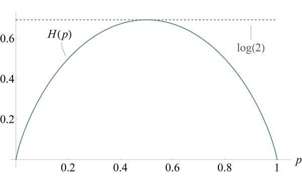
The binary entropy is zero in the deterministic case when $p$ is either one or zero. For these values the coin is either always heads or always tails; you know the outcome before the coin toss so gain no new information by observing the outcome. The maximum value of $\log(2)$ is attained when the $p=0.5$ and the distribution is as 'random' as possible.

The volume of a random variable #

In this section we show that entropy gives us the volume' occupied by a probability distribution, the so-called geometric interpretation of information theory [Wil17,§2]. Entropy was introduced by Claude Shannon as a tool of the information age [Sha48], when messages were being transmitted as binary sequences of zeros and ones. We will consider an example along these lines, so it will be convenient to take our logarithms to be in base two which we indicate with a subscript.

Suppose our random variable $A$ represents a letter in some alphabet, and sampling this multiple times gives us a message we wish to transmit. The probability distribution of $A$ is the relative frequency with which each letter is used. This could be seen as a crude model for the written language, or $A$ may be the outcome of some experiment or sensor readout that we wish to transmit to someone else. Shannon's key insight was that the probability distribution of $A$ introduces a fundamental limit on how efficiently we may encode a message as binary — the more spread out' the distribution, the less efficient an encoding we may use.

We consider an alphabet made up of four letters: ${a,b,c,d}$. First suppose that in our language each occurred with equal frequency, so the probability distribution was uniform: $p_i=1/4$. In this case the entropy of $A$ is

$H_2(A)=4\times\left(-\frac{1}{4}\log_2\frac{1}{4}\right)=2,$

with the subscript in $H_2$' to denote the base 2 logarithm. If we wish to encode a message in binary, Shannon's fundamental result was to show that we would need $H_2(A)$ bits per character [Sha48] — the higher the entropy, the less efficient an encoding we can achieve. We will take this on faith here, for a discussion on how to make this argument see [Wil17,§2.1]. One way of encoding the outcome of $A$ is
$\{(a,00),(b,01),(c,10),(d,11)\},$

in which case a message $aaba$ would be $00000110$. If $A$ is uniformly distributed then two bits per character is the best we can do.

Letters do not however appear with equal frequency, and we may use this structure to create a more efficient encoding. As an extreme example consider a different language $B$ with the same four letters, but suppose that $a$ occurred $97\%$ of the time — while $b$, $c$, and $d$ each had probability $1\%$. We could then use the code

$\{(a,0),(b,100),(c,101),(d,111)\},$

which would encode $aaba$ as $001000$. The number of bits used per letter now varies, but a string of ones and zeros can still be unambiguously decoded. A 0 represents an 'a', while a 1 means that the next two bits will tell you if it is a 'b', 'c', or 'd'. Since $a$ appears more frequently, $97\%$ of the time we would only use a single bit. The expected number of bits per character with this encoding is then $0.97\times 1+0.01\times 3\times 3=1.06$ (thanks u/CompassRed for pointing out a missing 3), so this code is twice as efficient as what we had for $A$. Calculating the entropy we find $H_2(B)\approx 0.24$, so we are still about four times less efficient than the optimal code. One way do to better would be to encode multiple characters at a time. Since '$a$' occurs so often we might let $0$ represent the sequence 'aaa', and this way the average bits per letter would be less than one.

The two random variables $A$ and $B$, despite occupying the same sample space, ended up having very different sizes. We would require two bits per character to transmit $A$ as a binary signal, as opposed to only $0.24$ for $B$. This 'size' is determined by the probability distribution, and quantified by the entropy. Thinking about random variables in this manner is called the geometric interpretation of entropy.

In this picture we see our random variable as occupying a sub-volume of the sample space due to the structure of its probability distribution. It may seem strange for us to use the word volume' for a discrete random variable, when we really mean 'number of points'. Points, length, area, and our usual three-dimensional 'volume' are all ways of measuring 'sizes', and which one is relevant depends on the dimension of problem at hand. In this series we will use the word 'volume' to refer to all of them. As we will discuss later this can all be made rigorous through the lens of measure theory (or see §5.2 of my thesis if you are impatient).

The volume occupied by a random variable is found by exponentiating the entropy to the power of whichever base we took our logarithm in.

1. In the example just covered $2^{H_2(A)}=2^2=4$, and so the random variable $A$ — which is uniformly distributed — occupies the entire sample space.
2. Suppose we had a variable $C$ which always used the letter $b$ with probability one. We would have $H_2(C)=0$, and $2^{H_2(C)}=2^0=1$. The variable occupies only a single letter as expected. For our variable $B$ we have $2^{H_2(B)}=2^{0.24}\approx 1.18$, so this occupies only slightly more than a single letter.
3. If a variable $C'$ were evenly distributed between $a$ and $b$ with probability $1/2$, the entropy would be
   $-\frac{1}{2}\log\frac{1}{2} -\frac{1}{2}\log\frac{1}{2}=\log 2,$
   and $2^{H_2(C')}=2^2=2$, occupying exactly two letters out of the sample space. (Thanks to @KevinSafford, u/Avicton and u/inetic for fixing typos.)

If we return to the binary entropy of a biased coin, the sample space has two elements: heads and tails. Exponentiating $H(p)$ gives

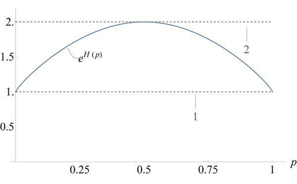
We can see that in the deterministic case where $p=0$ the random variable occupies a single element, either heads or tails. The full sample space is occupied when the coin is as random as possible, at $p=0.5$.

Let us briefly discuss the role of the base two logarithm. The final volumes are exactly the same as if we used the natural logarithm, since:

$2^{H_2(A)}=e^{H(A)}.$

The only role of base two was the intermediate step, when we interpreted $H_2(A)$ as the number of bits required to transmit each character. This was because we were signalling in binary — if we were sending our signals in trinary for example (with three 'trits' rather than two 'bits') then we would have had to reach for the base three logarithm instead.

Often in literature base two is used, reflecting the role of information theory in studying digital communications. We however don't want to study transmitting information in binary, but rather how the volume of a random variable changes as we gain information. In so far as any basis is natural, we may as well choose the natural logarithm in base $e$.

Conclusion #

In the geometric picture we visualise a random variable $A$ as occupying a sub-volume of its sample space, which is given by $e^{H(A)}$. A uniform distribution is spread out evenly over the entire sample space, while a deterministic random variable occupies only a single point.

In future posts we will see that the geometric picture offers a nice way to unify the entropy of a continuous and discrete random variable. All that you need to do is switch your idea of size from the discrete 'number of points' to the continuous analogues of 'length', 'area', or three-dimensional 'volume'. This will be particularly useful when we want to describe the interaction between continuous and discrete quantities. In the quantum example I discussed at the start, the measurement $M$ has discrete outcomes, from which we want to infer the continuous value of the magnetic field.

The next post will discuss correlations between random variables, such as when you observe a measurement $M$ to try and learn about some parameter $\Phi$. We will see how the volume of sample space occupied by the random variable shrinks as you gain more information about it, until it collapses to a single point with perfect information.

Let me know if you have any questions or comments about this article. Follow @ruvi_l on twitter for more posts like this, or join the discussion on Reddit:

Notes and further reading #

• u/lquant suggested David MacKay’s book 'Information Theory, Inference, and Learning Algorithms' for good coverage of the geometric interpretation.
• u/floormanifold pointed out that the geometric interpretation comes rigorously from something called the Asymptotic Equipartition Property. A nice 'less-rigorous' discussion of this is given in [Wil17,§2].

References #

[Wil17] Wilde, M. (2017). Quantum information theory (Second Edition). Cambridge University Press.

[CT05] Cover, T. M., & Thomas, J. A. (2005). Elements of Information Theory. In Elements of Information Theory. John Wiley & Sons. https://doi.org/10.1002/047174882A

[Sha48] Shannon, C. E. (1948). A mathematical theory of communication. The Bell System Technical Journal, 27(3), 379-423. https://doi.org/10.1002/j.1538-7305.1948.tb01338.x

---

• Next: Geometric interpretation of continuous entropy
• Previous: Electromagnetic transfer matrix at a boundary