Introduction #
In a previous post we looked at the geometric meaning of Maxwell's equations:
The key thing to remember was: if you see a divergence draw a three-dimensional volume and use the divergence theorem, while if you see a curl draw a two-dimensional surface and use Stokes' theorem. We are going to use this to derive the electromagnetic boundary conditions. Hopefully by the end of this they should seem pretty intuitive, and you will be able to quickly the boundary conditions them just by looking at Maxwell's equations.
Now things are complicated by the fact that if we are not in a vacuum, the electric and magnetic fields can induce extra charges and currents in the surface, which induce new fields, which induce even more charges and currents, and so on. For this reason it is convenient to write some of the equations in terms of and , because then only the `free' charges and currents , the ones that are put in at the start rather than induced by the fields, show up:
Deriving the boundary conditions #
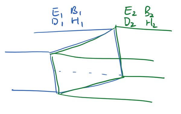
Let's suppose we have a boundary between two media, and some sort of electromagnetic wave propagates between the two. We want to know how the fields on one side relate to the fields on the other.
We will look at the conditions imposed on the fields by each of Maxwell's laws.
Gauss' Law for the Magnetic Field #
For our first candidate we will look at
There is a divergence, so that means we want to draw a three-dimensional box on both sides of the boundary, and use the divergence theorem to convert the left hand side to an integral of over the surface.
We have a solid rectangular box. The blue face lies inside the left region, the green face inside the right region, while the black faces cross both regions. Integrating both sides of Gauss' Law gives that the integral of over all six faces is equal to zero:
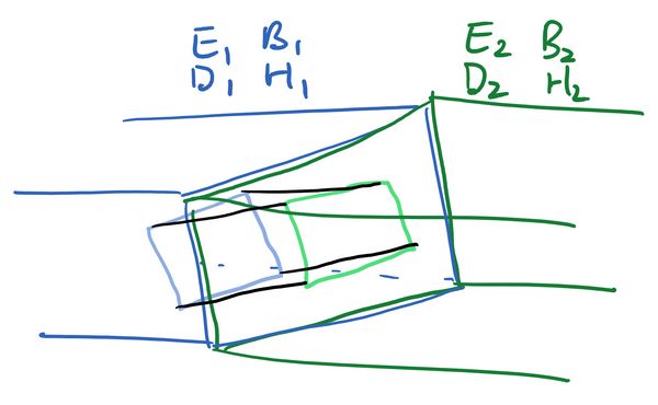
Let's suppose the blue and green faces have some area . Note that the unit normal has opposite sign on each side of the box, so it is pointing against but with . On the blue and green faces, taking the dot product with the unit normal selects the components of the magnetic field which are perpendicular to the boundary. We then have:
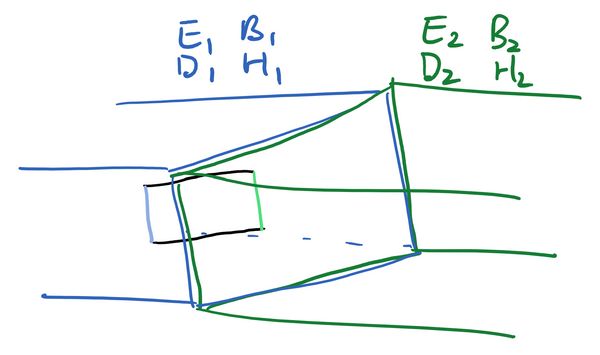
The integral over the black faces is annoying because each face has contributions from both and , so it doesn't have a nice answer. We can get rid of these parts though by making the box extremely thin. We bring the blue and green face closer together, shrinking the black faces to zero area while keeping the areas of the blue and green faces at . With this we will have
Dividing through by area then gives
In other words, the perpendicular component of the magnetic field is unchanged across the boundary. Since the perpendicular component of the magnetic field is , another way of writing this boundary condition is
Gauss' Law for the Electric Field #
Now we will analyse
The analysis for the left hand side is identical to what we had for the magnetic field, and we end up with
On the right hand side however the volume integral of over the box will be equal to the enclosed free charge. Let's assume there is a charge density per unit area on the boundary, then the right hand side will be , and we will have
or
As before we may re-write this as
Let's consider a special case. Suppose there is no free charge on the boundary (), and we are in linear media, so and . In this case the boundary condition becomes:
and we see that the normal component of the electric field is discontinuous across the boundary. The intuition for this is that the electric fields induce a bound charge density on the boundary, which causes the normal component of the electric fields to be discontinuous.
Faraday's Law #
We're done with the divergences, so let's move onto the simpler one of the curl equations:
Since we have a curl, this time we will draw a two-dimensional surface and then use Stokes' theorem.
Now the blue line lies inside the left material, the green line inside the right material, and the black lines cross the boundary and lie in both materials. We integrate both sides of Faraday's law over this surface. For the left hand side Stokes' theorem converts the integral of the curl over this surface to the line integral around the boundary:
Suppose the blue and green lines have length , then the line integrals over these become the parallel component of multiplied by , with again a sign difference because the line integral is pointing down on the blue side and up on the green side (as it goes anticlockwise around the rectangle)
Again the integrals over the black line are annoying, as each line crosses between the two regions. But again the cure is the same, to move the blue and green lines closer together (keeping them at length ), squeezing the rectangle thinner and thinner until the lengths of the black lines go to zero. In this case the integral over the black lines vanishes and we have
For the right hand side we want to integrate over the face of the rectangle. However we just squeezed the rectangle infinitely thin, so we will be integrating this over zero area, which will give us zero. The net result is
and then dividing by we find that the parallel component of the electric field is continuous across the boundary. Since the parallel component is the part perpendicular to the normal vector, we can also write this as
Ampère's Law #
This one is left as an exercise to the reader! Begin with
and show that you end up with
where is the surface current density. If there is no free current and we are in a linear material (), this becomes
Conclusion #
There you have it! Once you understand the general principle, you can read off the boundary conditions very quickly by just looking at Maxwell's laws:
The divergence laws will tell you about the perpendicular components, while the curl laws tell you about the parallel. The homogenous (source-free) laws give you continuity (the same fields on either side), while the inhomogeneous laws lead to discontinuity (factors of and on either side). After a bit of thinking you should be able to jump straight to