Introduction #

In this post we'll go through a very useful technique for solving linear differential equations: the differential operator method. Though the name is a bit of a mouthful (if you've seen a better one please let me know!), the underlying principle is about using intuition and techniques from polynomials to solve linear differential equations. I'll be applying this to equations that arise in RC circuits, but won't assume any knowledge of electronics.

Most examples on the internet use the differential operator method to find exact solutions. However, in physics we are almost always interested in approximations. Exact solutions do not exist for a general differential equation. Moreover, a simple approximation can help us understand the behaviour of a circuit better than a complicated exact expression.

In this post we will look at two different circuits, with equations:

$\begin{aligned}V_R(t)+RC\frac{\mathrm{d}V_R(t)}{\mathrm{d}t}&=RC \frac{\mathrm{d}V_{in}(t)}{\mathrm{d}t}, \\ \frac{\mathrm{d}V_C(t)}{\mathrm{d}t}+\frac{1}{RC} V_C(t)&=\frac{1}{RC} V_{in}(t).\end{aligned}$

In the above $V_{in}(t)$ is the input voltage, $V_R(t),V_C(t)$ are the output voltages that we measure, and $R,C$ the resistance and capacitance of the circuit. Using the operator method we will be able to derive the approximate solutions:

$\begin{aligned}V_R(t) &\approx RC\frac{\mathrm{d}V_{in}(t)}{\mathrm{d}t}+(RC)^2\frac{\mathrm{d}^2V_{in}(t)}{\mathrm{d}t^2}, \\ V_C(t)&\approx\frac{1}{RC}\int_0^tV_{in}(t')\mathrm{d}t \\ &\phantom{=}+\frac{1}{(RC)^2}\int_0^{t}\left(\int_0^{t'}V_{in}(t'')\mathrm{d}t''\right)\mathrm{d}t'.\end{aligned}$

By making $RC$ sufficiently small in the first circuit, and large in the second, we can consider only the first term on the right hand sides. These circuits can be used as integrators or differentiators — no computer required! As we discuss at the end, circuits like this can be much faster (and definitely smaller & cheaper) than a computer, so are very useful for applications such as feedback control.

Our coverage of the operator method will be brief, and focused on solving the two equations above. More details on the method can be found in [C18]. I also won't go into the details of electrical circuits, and what a resistor and capacitor are. I tried to write the post so that you can just follow the maths regardless. If you can't, please let me know what I've missed or what doesn't make sense! For a detailed introduction to RC circuits you can check out [HH15,§1.12-15]

The differential operator method #

Let's begin by introducing the operator $D$, which is just an abbreviation of the derivative with respect to $t$:

$\frac{\mathrm{d}}{\mathrm{d}t}f(t)=Df(t).$

We then have

$\begin{gathered}Dt^3=3t^2,\\De^{3t}=3e^{3t},\\ D\cos(2t)=-2\sin(2t).\end{gathered}$

Higher order derivatives are represented by powers of $D$:

$\begin{gathered}D^2\left(4t^2-t^3\right)=8-6t,\\ D^3e^{at}=a^3e^{at},\end{gathered}$

where in the last line $a$ is any variable.

We can also add, subtract, and multiply $D$ just as if it were a variable:

$\left(1-2D+aD^2\right)\sin(\omega t)=\sin(\omega t)-2\omega\cos(t)-a\omega^2\sin(\omega t).$

Here comes the fun part. Suppose you want to solve the differential equation:

$f(t)+af'(t)=g(t),$

where $a$ is a constant, $g$ is known, and $f$ is the function you want to find. Writing the derivative as an operator, we can just solve for $f$:

$\begin{gathered}(1+aD)f(t)=g(t), \\ f(t)=\frac{1}{1+aD}g(t).\end{gathered}$

We are dividing by the derivative! In fact, we will go one step further, and use the Taylor series

[eqTaylorExpansion]: $\frac{1}{1-x}=1+x+x^2+\cdots.$

Setting $x=-aD$, we obtain the solution as an infinite sum:

$f(t)=\sum_{n=0}^{\infty}(-1)^na^nD^ng(t).$

If $a$ is a small number (i.e. $0.01$), then $a^2$ is much smaller ($0.0001$), and $a^3$ will be so small as to be negligible. This gives us an approximate solution:

$f(t)\approx -ag'(t)+a^2g''(t).$

If $a$ is not small you have a couple of options.

• You might be able to explicitly compute the sum if $g(t)$ is 'nice' (see the appendix for an example).
• By thinking about the problem a bit more you can often get a solution without having to compute the sum, see [C18].

A natural question to ask is how we should interpret $\frac{1}{D}$? Since

$D\left(\frac{1}{D}\right)=\frac{D}{D}=1,$

then $1/D$ must 'cancel out' the derivative $D$. This is the integral:

$\begin{gathered}\frac{1}{D}\left(1+2t-at^4\right)=t+t^2-\frac{a}{5}t^5,\\ \frac{1}{D}\sin(\omega t)=-\frac{1}{\omega}\cos(\omega t).\end{gathered}$

There are a couple of points we should discuss before we move on. Firstly, I mentioned that the derivative operator method is useful for equations that are linear in $f$. That is:

• There are no derivatives of $f$ multiplied together, such as $\left(f'(t)\right)^2$ or $f'(t)f''(t)$.
• You don't have $f$ or a derivative multiplied by time: $tf'(t)$.

The solution method relies on pulling out all the derivatives, so that you can write the equation as $f(t)$ multiplied by a polynomial of $D$. Try and convince yourself that this isn't possible if the equation isn't linear.

Secondly, we have played fast and loose with mathematical rigour. If you thought treating the derivative $\frac{\mathrm{d}y}{\mathrm{d}t}$ as a fraction was bad, what about Taylor expanding $\frac{1}{1+a(\mathrm{d}/\mathrm{d}t)}$? It is right to be concerned about these things, since asking such questions makes you more aware of the limits of the techniques you are using. I won't dive deep into the rigor here, but do justify our expansions somewhat in the appendix. For more details see [C18].

RC differentiator #

Let's consider the electric circuit formed by connecting a time-dependent voltage source $V_{in}(t)$ to a capacitor and resistor in series:

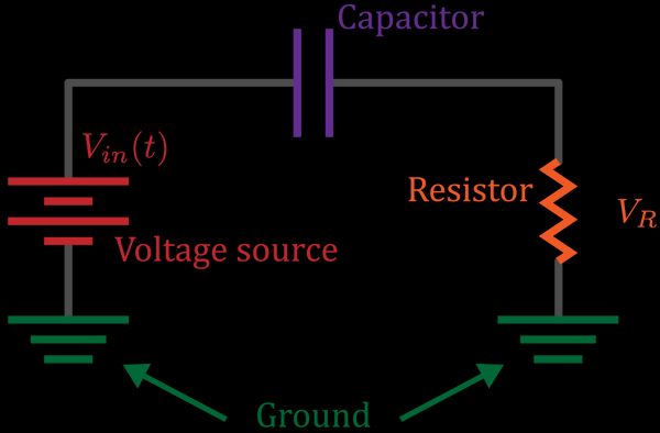
In the appendix we show that the voltage $V_R(t)$ across the resistor has differential equation

$V_R(t)+RC\frac{\mathrm{d}V_R(t)}{\mathrm{d}t}=RC\frac{\mathrm{d}V_{in}(t)}{\mathrm{d}t},$

where $R$ and $C$ are the resistance and capacitance respectively (if you are unfamiliar with electronics feel free to skip the derivation). Suppose the resistor and capacitor have been chosen so that the the product $RC$ is 'small' — see the appendix for a discussion on exactly what 'small' means. In that case we will abbreviate

$\epsilon=RC,$

and re-write the differential equation in operator notation:

$\left(1+\epsilon D\right)V_R=\epsilon DV_{in}.$

We can solve this using the Taylor series as before:

$\begin{aligned}V_R &=\frac{1}{1+\epsilon D}\epsilon DV_{in},\\ &=\left(1-\epsilon D+\epsilon^2D^2-\cdots\right)\epsilon DV_{in}, \\ &=\left(\epsilon D-\epsilon^2D^2+\cdots\right)V_{in}.\end{aligned}$

This sum will go on forever. However since $\epsilon$ is small, we can get a good approximation from just the first couple of terms. The biggest contribution will be

$V_R(t)\approx\epsilon DV_{in}=RC\frac{\mathrm{d}V_{in}(t)}{\mathrm{d}t},$

Thus voltage across the resistor will approximately equal the derivative of the input voltage. The second term in the sum gives us a correction $-(RC)^2V''_{in}(t)$, which will be negligible if $RC$ is small enough.

RC integrator #

The same circuit can also be used to construct an integrator. All of the methods are the same as the last part, so I encourage you to try and work through this on your own. This time we measure the voltage drop across the capacitor:

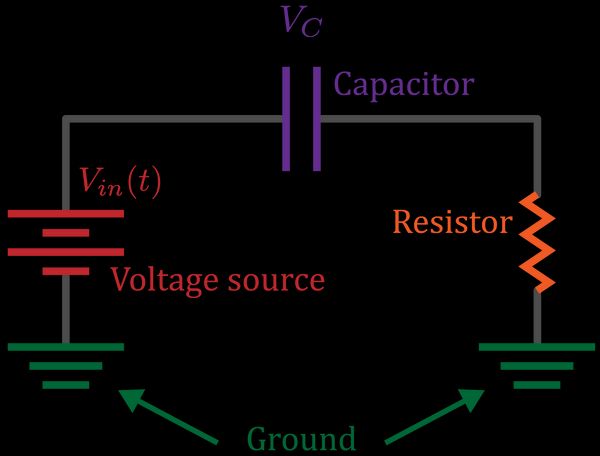
In the appendix we show that this has equation

$\frac{\mathrm{d}V_C}{\mathrm{d}t}+\frac{1}{RC}V_C=\frac{1}{RC}V_{in}.$

This time we will suppose that $RC$ is large, so let's set

$\epsilon=\frac{1}{RC}.$

Re-writing in terms of differential operators, we derive

$\begin{aligned}\left(D+\epsilon\right)V_C &= \epsilon V_{in},\\ V_C&=\frac{1}{D+\epsilon}\epsilon V_{in}.\end{aligned}$

We want to apply the Taylor expansion [eqTaylorExpansion], which requires the denominator of the fraction to be $(1+x)$ for small $x$. We thus re-write this as

$\begin{aligned}V_C &= \frac{1}{D}\frac{1}{1+\epsilon D^{-1}}\epsilon V_{in}, \\ &= D^{-1}\left(1-\epsilon D^{-1}+\epsilon^2D^{-2}-\cdots\right)\epsilon V_{in}.\end{aligned}$

The largest term will then be

$\begin{aligned}V_C &= \epsilon D^{-1}V_{in}, \\ &=\frac{1}{RC}\int_0^t V_{in}(t')\mathrm{d}t',\end{aligned}$

so this circuit computes the integral. The next largest term will be the double integral:

$-\frac{1}{(RC)^2}\int_0^{t}\left(\int_0^{t'}V_{in}(t'')\mathrm{d}t''\right)\mathrm{d}t'.$

That looks very fancy! But it was quite straightforward to derive using the operator method.

Discussion #

I hope this post has convinced you of the power of the differential operator method. Using just a bit of algebra and a Taylor expansion, we solved some quite complicated-looking differential equations. Moreover these weren't artificial textbook problems, they describe the behaviour of real circuits. We've only just scratched the surface here, and I recommend searching the internet or checking out [C18] for more details.

The circuits we analysed are examples of analog computers. Analog computation is a fascinating subject, and I recommend checking out this Veritasium video to see what we were capable of before the modern digital age. Did you know Lord Kelvin devised a machine that could do the Fourier transform, and so accurately predict the tides, in 1872? It's descendants were still being used up until the 1960s!

Even today, analog circuits are very useful. For simple applications they will always be much smaller and cheaper than a computer. Moreover, computers are digital, working with lists of ones and zeros. In a laboratory however most signals are analog, for example a sensor which produces a voltage proportional to the height of a levitated particle. If we want to differentiate this signal to find the velocity, we would first have to convert the continuous voltage (2.17V) to a binary sequence (1010111). Then if we want to apply feedback to the particle proportional to its velocity, we would have to convert the digital list of ones and zeros back to a voltage to send to our apparatus. The conversion process takes tens of microseconds, which is too slow for many applications. Thus for realtime feedback control, an electronic circuit which takes a time-varying voltage and returns the derivative of that voltage can be much more useful than a computer.

Have any comments or questions? Let me know! Follow @ruvi_l on twitter for more posts like this, or join the discussion on Reddit:

You can also feel free to send me an email.

Appendix #

Solving a differential equation #

Suppose we wish to solve the differential equation

$f(t)+af'(t)=3t^2-5t.$

We showed above that this can be written as

$f(t)=\sum_{n=0}^{\infty}(-1)^na^nD^n\left(3t^2-5t\right)$.

Only three terms in the sum will be nonzero, since $D^n(3t^2-5t)$ is zero when $n$ is greater than or equal to three. These terms are:

$\begin{aligned}n=0&: 3t^2-5t, \\ n=1&: -6at+5a, \\ n=2&: 6a^2. \end{aligned}$

Adding them together then gives the solution

$f(t)=3t^2-(5+6a)t+(6a^2+5a).$

Differentiator circuit equation #

Suppose we start at the ground on the left, and follow the circuit until we reach the ground on the right. The voltage starts at zero, is increased by the battery to $V_{in}(t)$, then falls by $V_C(t)$ across the capacitor and $V_R(t)$ across the resistor. Since the overall change in voltage over this path is zero — we begin and end at ground voltage — we have

$\begin{gathered}0 = +V_{in}(t)-V_R(t)-V_C(t), \\ V_C(t)=V_{in}(t)-V_R(t).\end{gathered}$

A capacitor consists of two metal plates facing each other. When a voltage $V_C$ is applied, charges $+Q$ and $-Q$ build up on the plates in proportion

$Q=CV_C,$

where $C$ is a constant called the capaciatance of the capacitor. Differentiating both sides of this with respect to time, and noting that current $I$ is the deriative of charge, gives

$\begin{aligned}I&=C\frac{\mathrm{d}V_C}{dt},\\ &= C\left(\frac{\mathrm{d}V_{in}}{\mathrm{d}t}-\frac{\mathrm{d}V_R}{\mathrm{d}t}\right).\end{aligned}$

The current $I$ flowing through the capacitor must be the same as the current flowing through the resistor (since there is nowhere else for current to go). Ohm's law $V_R=IR$ then gives

$V_R=RC\frac{\mathrm{d}V_{in}}{\mathrm{d}t}-RC\frac{\mathrm{d}V_R}{\mathrm{d}t}.$

This is a differential equation for the unknown $V_R(t)$ across the resistor, in terms of the applied signal $V_{in}(t)$.

Integrator circuit equation #

As before we start at the ground on the left, and move through the circuit to the ground on the right:

$\begin{gathered}0=+V_{in}-V_C-V_R, \\ V_R=V_{in}-V_C\end{gathered}.$

Across the capacitor we have

$I=C\frac{\mathrm{d}V_C}{\mathrm{d}t}.$

Substituting in Ohm's law $I=V_R/R$ then gives a differential equation for the voltage across the capacitor:

$\begin{gathered}\frac{1}{R}\left(V_{in}-V_C\right)=C\frac{dV_C}{dt}, \\ \frac{\mathrm{d}V_C}{\mathrm{d}t}+\frac{1}{RC}V_C=\frac{1}{RC}V_{in}. \end{gathered}$

Note that here we have written the equation in terms of $1/(RC)$. This is because the circuit behaves as an integrator when $RC$ is large, so $1/(RC)$ will be our small $\epsilon$.

The meaning of a big or small RC #

The product $RC$ has units of time, so its value will change depending on if we measure time in seconds, years, or nanoseconds. Choosing different units can't change the behaviour of our circuit! Therefore whenever you talk about the size of a quantity with units, what you really mean is that it is big or small compared to another quantity with the same units. So what is that other quantity?

Let's look at the differentiator first. We derived our approximation by Taylor expanding $1/(1+(RC)D)$, so what we really want is $(RC)D$ to be small. Note that the derivative $D=\frac{\mathrm{d}}{\mathrm{d}t}$ has units of inverse time, so the product $(RC)D$ is unitless. What we are saying then, is that $(RC)$, multiplied by the derivative of $V_{in}$, must be small. Noticeable changes in the input signal $V_{in}$ must take longer than a time $RC$ to occur. If $V_{in}$ is changing very quickly, we will need a much lower resistance and capacitance for the circuit to work.

Now let's consider the integrator. In this case the Taylor expansion requires $\frac{1}{(RC)D}$ to be small, so $(RC)D$ is large. In other words, our input signal $V_{in}$ must be changing relatively quickly, when compared to the time $RC$. If our input signal changes very slowly, we will need to use a higher resistor or stronger capacitor to integrate the signal.

References #

[C18] Chen, W. (2018). Differential Operator Method of Finding A Particular Solution to An Ordinary Nonhomogeneous Linear Differential Equation with Constant Coefficients arXiv:1802.09343.
[HH15] Horowitz, P. & Hill, W. (2015). The Art of Electronics (3rd edition). Cambridge: Cambridge University Press.

---

• Next: Connecting to a Red Pitaya
• Previous: Quadrature parameterisation for second-order bosonic Hamiltonians