Introduction #

... quaternions appear to exude an air of nineteenth century decay, as a rather unsuccessful species in the struggle-for-life of mathematical ideas. Mathematicians, admittedly, still keep a warm place in their hearts for the remarkable algebraic properties of quaternions but, alas, such enthusiasm means little to the harder-headed physical scientist.

— Simon L. Altmann, Rotations, Quaternions, and Double Groups

This article was written together with Ang Chen Ye.

Early in physics, we learn to model the motion of point particles. We do this by assigning Euclidean coordinates $x,y,z$, and finding differential equations for their evolution. However, in everyday life we rarely encounter point particles. Instead we are surrounded by rigid bodies. While these have a centre of mass that behaves like a point particle, they can also do things like twist and spin. So to model a rigid body, we need coordinates that can describe all of their degrees of freedom.

In this article we will use quaternions to describe the motion of rigid bodies. Euler's equations were re-written in quaternion form in [CR04]. Here we will use [LM18] to generalise this to full Lagrangian mechanics on the quaternions.

All images in this article were created in Blender. You can use them for your own purposes, but please reference this article.

This article may be a bit harder to follow than the other articles on this site, as we haven't had time to explain everything in detail. Recommended background reading is [LM18]. If you have any questions, feel free to email me@ruvi.blog.

Euler angles, and their failures #

We will use coordinates $x,y,z$ to describe the position of the centre of mass. On top of these, we need some more coordinates to describe the orientation of the body. A common way to do this is Euler angles. These are three angles, representing a series of rotations that transform the body from its initial orientation to its current one:

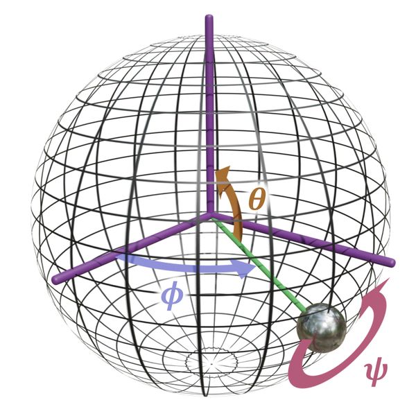
In the image above, the rigid body is a spherical pendulum, and the initial configuration is taken to be lying along the $z$-axis. This initial configuration is rotated first by $\psi$ about the $z$-axis, then $\theta$ about the $x$-axis, and finally $\phi$ about the $z$-axis again. These three Euler angles $\theta,\phi,\psi$ thus let us describe any orientation of the body. Adding in $x,y,z$ to describe the position pendulum's base, we see that we can describe any position and orientation using a total of six coordinates.

We won't go into it here, but we can find differential equations for all of the coordinates $x,y,z,\theta,\phi,\psi$, which allow us to solve for how the rigid body evolves in time. These are quite complicated. But even worse, the equations are singular. If we try and numerically simulate them, there are particular values for the Euler angles where if they are ever reached, the simulation will blow up. This is because, while $\theta,\phi,\psi$ should describe a three-dimensional parameter space, there are particular configurations where it collapses to two dimensions. In this situation the coordinates can no longer describe the full range of motion of the object, and the numerics do not survive. To see this, consider the image below:

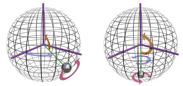
In the position on the left, varying either of the three angles will move the pendulum in a different way. It thus has three degrees of freedom. However if the pendulum lies straight down, varying $\phi$ and $\psi$ produce exactly the same motion. Our coordinate system has lost a degree of freedom, and can no longer describe the full range of motion of the pendulum.

Failure of Euler angles stems fundamentally from geometry. The orientation of a rigid body has a naturally spherical geometry. However when we write down three angles $\theta,\phi,\psi$, we are using Euclidean flat space to parameterise this curved geometry. Such a thing can only be done locally, and will always result in a singularity somewhere.

If we want to avoid singularities, we need to find a way to parameterise rigid bodies using a space whose geometry is also curved. We'll see that that the unit quaternions are up to the task.

Crash course in quaternions #

To form the complex numbers, we add a number $i$ with the rule $i^2=-1$. For quaternions, we add three numbers $i,j,k$. These also square to minus one:
$i^2=j^2=k^2=-1.$
Moreover, their products with each other are
$ij=k,\;jk=i,\;ki=j.$
One big difference from the complex numbers is that multiplication is no longer commutative. $i,j,k$ anti-commute with one another:
$ji=-k,\;kj=-i,\;ik=-j.$
Real numbers however do commute with $i,j,k$. These rules are all we need to know to do computations with the quaternions.

The conjugate of a quaternion is defined similarly to the complex numbers. If
$q=q_0+iq_1+jq_2+kq_3$
where $q_0,\ldots,q_3$ are real numbers, then
$q^*=q_0-iq_1-jq_2-kq_3.$
The norm of the quaternion is then
$\lVert q\rVert^2=q^*q=q_0^2+q_1^2+q_2^2+q_3^2.$
If $q$ is a unit quaternion, then $q^{-1}=q^*$.

Let's introduce a bit of notation to make handling quaternion expressions a bit easier. For a quaternion
$q=q_0+iq_1+jq_2+kq_3,$
we'll refer to $q_0$ as the real part. If the real part is zero, we say that $q$ is a pure quaternion. We may abbreviate this as
$q=(q_0,\vec{q}),$
where $\vec{q}=(q_1,q_2,q_3)$.

We'll now give a few identities that are useful for quaternion computations. We won't prove any of them here, but it's a good exercise to try and do so using the quaternion rules given above.

Mutliplication rule #

[eqQuaternionMultiplication]: $(q_1,\vec{q}_1)(q_2,\vec{q}_2)=\left(q_1q_2-\vec{q}_1\cdot\vec{q}_2,\;q_1\vec{q}_2+q_2\vec{q}_1+\vec{q}_1\times\vec{q}_2\right).$
To see this just expand everything out.

Cross product #

If $\vec{u},\vec{v}$ are pure quaternions, then
[eqCrossProduct]: $\vec{u}\vec{v}-\vec{v}\vec{u}=2\vec{u}\times\vec{v}.$
This follows from [eqQuaternionMultiplication]

Rotations #

Suppose $\hat{u}$ is a unit vector in $\mathbb{R}^3$. Then the quaternion
$q=\left(\cos(\theta/2),\sin(\theta/2)\hat{u}\right)$
represents a rotation about the axis $\hat{u}$ by an angle $\theta$. What this means is that if $\vec{v}$ is a pure quaternion, and
$\vec{w}=q\vec{v}q^{-1},$
then $\vec{w}$ is a pure quaternion corresponding to the rotated $\vec{v}$. For proof see section 5 of [CR04].

Inner product #

The inner product on the quaternions is defined as
$\langle p,q\rangle=\frac{1}{2}\left(p^*q+q^*p\right).$
Note that this is symmetrised to account for non-commutativity of quaternions. We can also write this as
$\langle p,q\rangle=\mathrm{Re}(pq).$
For $p=(p_0,\vec{p})$, $q=(q_0,\vec{q})$, we have
$\langle p,q\rangle=p_0q_0+\vec{p}\cdot\vec{q}.$

If $u$ is any other quaternion, we have
$\langle p,uq\rangle=\frac{1}{2}\left(p^*uq+q^*u^*p\right),$
$=\frac{1}{2}\left((u^*p)^*q+q^*(u^*p)\right),$
$=\langle u^*p,q\rangle.$

Quaternion description of a rigid body #

Orientation and its derivative #

We will represent the orientation of the rigid body with a unit quaternion representing the rotation taking the body to that position:
$q=\left(\cos(\theta/2),\sin(\theta/2)\hat{u}\right).$
This provides a one-to-one correspondence between orientations and unit quaternions.

We also need to represent the rate of change of orientation. This is a tangent vector at $q$. Let $q(t)$ be a curve on the sphere, then
$q(t)^*q(t)=1.$
Differentiating both sides, and labelling $v=\dot{q}$ as the velocity, gives
[eqTangentCondition]: $v^*q+q^*v=0.$
Any quaternion $v$ satisfying this equation is a tangent vector at $q$, representing some angular velocity relative to the configuration $q$.

Let's try and interpret $v$ physically, following section 8.2 of [CR04]. Suppose
$q=q_0+\vec{q}.$
Then
$q^*=q_0-\vec{q},$
and
$v=v_0+\vec{v},$
where $v_0,\vec{v}$ are the derivatives of $q_0,\vec{q}$ with respect to time. The scalar part of $q^*v$ is
$q_0v_0+\vec{q}_0\cdot\vec{v}_0=q_0\frac{\mathrm{d}q_0}{\mathrm{d}t}+\vec{q}\cdot\frac{\mathrm{d}\vec{q}}{\mathrm{d}t},$
$=\frac{1}{2}\frac{\mathrm{d}}{\mathrm{d}t}\lVert q\rVert^2,$
$=0,$
where the last line follows since $q$ is a unit quaternion with constant norm. Thus $q^*v$, and its conjugate $v^*q$, are pure quaternions.

Angular velocity #

Let's define this pure quaternion as
[eqDefomega]: $\omega=2vq^*.$
Note that the factor of $2$ is added for convenience based on what will come later. Then
[eqvomega]: $v=\frac{1}{2}\omega q.$

Let $x$ be a vector in the lab frame, and $X$ the corresponding vector in the body frame. Then
$x=qXq^*.$
The derivative is
$\dot{x}=vXq^*+qXv^*,$
$=\frac{1}{2}\left(\omega qXq^*+qXq^*\omega^*\right),$
$=\frac{1}{2}\left(\omega x-x\omega\right),$
where the last line follows since $\omega$ is a pure quaternion. From [eqCrossProduct] we find
$\dot{x}=\vec{\omega}\times\vec{x}.$
This shows that physically, $\vec{\omega}$ represents the angular velocity of the rigid body, as viewed in the lab frame. For example if $\vec{\omega}=\omega_z\hat{z}$, then the body is rotating about the lab's $z$-axis.

Alternate angular velocity #

Alternatively, we could have defined the angular velocity as
[eqDefOmega]: $\Omega=2q^*v,$
and consequently
[eqvOmega]: $v=\frac{1}{2}q\Omega.$
In terms of this a vector $x$ evolves as
$\dot{x}=vXq^*+qXv^*,$
$=\frac{1}{2}\left(q\Omega Xq^*+qX\Omega^*q^*\right),$
$=\frac{1}{2}q\left(\Omega X-X\Omega\right)q^*,$
$=q\left(\Omega\times X\right)q^*.$
Thus $\Omega$ gives the angular velocity with respect to the body frame. If $\Omega=\Omega_z\hat{z}$, this means that the body is rotating about its own $z$-axis.

We can work with either $\omega$ or $\Omega$. However when trying to work out the rotational kinetic energy of the body, $\Omega$ is more useful. So going forward we will use this.

Euler-Lagrange equations #

Suppose we write down a Lagrangian in terms of the quaternion position $q$ and angular velocity $\Omega$. What are the Euler-Lagrange equations, that give us the equations of motion? From before we have
[eqqDot]: $\dot{q}=\frac{1}{2}q\Omega.$
What remains is to find the equation for $\dot{\Omega}$. This will require us to develop variational calculus on the quaternions. We will do this by applying the Lie group formalism in section 8.6 of [LM18].

Infinitesimal variations #

Suppose $q(t)$ is a path, and let $q^{\epsilon}$ be a variation of this. We need a way of parameterising this in terms of a Euclidean variation. In general we can write
$q^{\epsilon}(t)=q(t)e^{\epsilon\eta(t)},$
where $\eta(t)$ is an arbitrary pure quaternion such that $\eta(t_0)=\eta(t_f)=0$. To find the corresponding tangent vector, we must differentiate the product $q(t)e^{\epsilon\eta(t)}$ with respect to time. Evaluating this derivative is complicated by the fact that since we are dealing with quaternions, $q(t),\eta(t),\dot{\eta}(t)$ will not in general commute. We can get around this by Taylor expanding the exponential:
$q^{\epsilon}=q(t)+\epsilon q(t)\eta(t)+\mathcal{O}(\epsilon^2).$
Then
$\dot{q}^{\epsilon}(t)=\frac{\mathrm{d}}{\mathrm{d}t}q^{\epsilon}(t),$
$=\dot{q}(t)+\epsilon \dot{q}(t)\eta(t)+\epsilon q(t)\dot{\eta}(t)+\mathcal{O}(\epsilon^2).$
The angular velocity [eqDefOmega] is then
$\Omega^{\epsilon}(t)=2q^{*\epsilon}\dot{q}^{\epsilon},$
$=2\left(q^*-\epsilon \eta q^*\right)\left(\dot{q}+\epsilon\dot{q}\eta+\epsilon q\dot{\eta}\right)+\mathcal{O}(\epsilon^2),$
$=2q^*\dot{q}+2\epsilon\left(-\eta q^*\dot{q}+q^*\dot{q}\eta+q^* q\dot{\eta}\right)+\mathcal{O}(\epsilon^2),$
where we have used $\eta(t)^*=-\eta(t)$ since $\eta(t)$ is a pure quaternion. This gives us
$\Omega^{\epsilon}(t)=\Omega(t)+\epsilon\left(\Omega(t)\eta(t)-\eta(t)\Omega(t)+2\dot{\eta}(t)\right)+\mathcal{O}(\epsilon^2).$

Now let us calculate the effect of an infinitesimal variation, when $\epsilon$ is very small. The variation in orientation is
$\delta q=\left.\frac{\mathrm{d}}{\mathrm{d}\epsilon}q^{\epsilon}\right\rvert_{\epsilon=0},$
which gives
[eqDeltaq]: $\delta q=q\eta,$
[eqDeltaqstar]: $\delta q^*=-\eta q^*.$
The variation in angular momentum is
$\delta \Omega=\left.\frac{\mathrm{d}}{\mathrm{d}\epsilon}\Omega^{\epsilon}\right\rvert_{\epsilon=0},$
$=\Omega(t)\eta(t)-\eta(t)\Omega(t)+2\dot{\eta}.$
Thus we find
[eqDeltaOmega]: $\delta\Omega=[\Omega,\eta]+2\dot{\eta}.$

With these, we can parameterise an arbitrary variation using a pure quaternion $\eta$. This lets us turn the problem into one of unconstrained optimisation, since $\eta$ is an arbitrary three-dimensional vector.

Variation in the action #

Now suppose we have a Lagrangian
$\mathcal{L}(q,q^*,\Omega)=T(q,q^*,\Omega)-U(q,q^*).$
Note that our Lagrangian will be a function of both $q,q^*$, since both of these are used in the quaternion rotation formula. We want to find the trajectory $q(t),\Omega(t)$ which minimises the action
$\mathcal{S}=\int\mathcal{L}(q,q^*,\Omega)\mathrm{d}t.$

Let us consider an arbitrary variation
$\mathcal{S}^{\epsilon}=\int\mathcal{L}(q^{\epsilon},q^{*\epsilon},\Omega^{\epsilon})\mathrm{d}t.$
Then
$\delta\mathcal{S}=\int\left[\left\langle\frac{\partial\mathcal{L}}{\partial q},\delta q\right\rangle+\left\langle\frac{\partial\mathcal{L}}{\partial q^*},\delta q^*\right\rangle+\left\langle\frac{\partial\mathcal{L}}{\partial\Omega},\delta\Omega\right\rangle\right]\mathrm{d}t.$
Into this we substitute [eqDeltaq], [eqDeltaqstar], and [eqDeltaOmega]. The first term is
$\left\langle\frac{\partial\mathcal{L}}{\partial q},\delta q\right\rangle=\left\langle\frac{\partial\mathcal{L}}{\partial q},q\eta\right\rangle,$
$=\left\langle q^*\frac{\partial\mathcal{L}}{\partial q},\eta\right\rangle.$
The second term is
$\left\langle\frac{\partial\mathcal{L}}{\partial q^*},\delta q^*\right\rangle=\left\langle\frac{\partial\mathcal{L}}{\partial q^*},-\eta q^*\right\rangle,$
$=\left\langle-\frac{\partial\mathcal{L}}{\partial q^*}q,\eta\right\rangle.$
The third term is (using integration by parts)
$\left\langle\frac{\partial\mathcal{L}}{\partial\Omega},\delta\Omega\right\rangle=\left\langle\frac{\partial\mathcal{L}}{\partial\Omega},\Omega\eta-\eta\Omega+2\dot{\eta}\right\rangle,$
$=\left\langle\Omega^*\frac{\partial\mathcal{L}}{\partial\Omega}-\frac{\partial\mathcal{L}}{\partial\Omega}\Omega^*,\eta\right\rangle+\left\langle-2\frac{\mathrm{d}}{\mathrm{d}t}\left(\frac{\partial\mathcal{L}}{\partial\Omega}\right),\eta\right\rangle,$
$=\left\langle\left[\Omega^*,\frac{\partial\mathcal{L}}{\partial\Omega}\right]-2\frac{\mathrm{d}}{\mathrm{d}t}\left(\frac{\partial\mathcal{L}}{\partial\Omega}\right),\eta\right\rangle.$
$=\left\langle\left[\frac{\partial\mathcal{L}}{\partial\Omega},\Omega\right]-2\frac{\mathrm{d}}{\mathrm{d}t}\left(\frac{\partial\mathcal{L}}{\partial\Omega}\right),\eta\right\rangle.$

Putting all this together we have
$\delta\mathcal{S}=\int\left\langle q^{*}\frac{\partial\mathcal{L}}{\partial q}-\frac{\partial{\mathcal{L}}}{\partial q^*}q+\left[\frac{\partial\mathcal{L}}{\partial\Omega},\Omega\right]-2\frac{\mathrm{d}}{\mathrm{d}t}\left(\frac{\partial\mathcal{L}}{\partial\Omega}\right),\eta\right\rangle\mathrm{d}t.$
If $q(t)$ is the actual trajectory, then the variation in the action $\delta\mathcal{S}$ is zero for all $\eta$. This gives us the Euler-Lagrange equations for the quaternions:
[eqOmegaDot]: $\frac{\mathrm{d}}{\mathrm{d}t}\left(\frac{\partial\mathcal{L}}{\partial\Omega}\right)=\frac{1}{2}\left(q^*\frac{\partial\mathcal{L}}{\partial q}-\frac{\partial\mathcal{L}}{\partial q^*}q+\left[\frac{\partial\mathcal{L}}{\partial\Omega},\Omega\right]\right).$

Examples #

Free body #

Let's now use this to derive Euler's equations for a free rigid body. The Lagrangian in Euclidean space is just the kinetic energy
$\mathcal{L}=\frac{1}{2}\vec{\Omega}^TI\vec{\Omega},$
where $I$ is the moment of inertia in the body frame. We need to re-write this in terms of quaternions.

Let $\Omega$ be the pure quaternion corresponding to $\vec{\Omega}$. Define $\mathcal{I}$ to be the $4\times 4$ matrix
$\mathcal{I}=\left(\begin{array}{cc} 0 & 0 \\ 0 & \mathcal{I}\end{array}\right),$
where $I$ is the $3\times 3$ inertia tensor. Then we have
$\mathcal{L}=\frac{1}{2}\langle\Omega,\mathcal{I}\Omega\rangle.$
Writing it out in components gives
$\frac{\partial\mathcal{L}}{\partial\Omega}=\mathcal{I}\Omega=I\vec{\Omega},$
so the left-hand side of Euler's equations is
$\frac{\mathrm{d}}{\mathrm{d}t}\left(\frac{\partial\mathcal{L}}{\partial\Omega}\right)=I\vec{\Omega}'.$
The right-hand side is
$\frac{1}{2}\left[\frac{\partial\mathcal{L}}{\partial\Omega},\Omega\right]=\vec{\frac{\partial\mathcal{L}}{\partial\Omega}}\times\vec{\Omega},$
$=(I\vec{\Omega})\times\vec{\Omega}.$

Thus we get
$I\vec{\Omega}'=(I\vec{\Omega})\times\vec{\Omega}.$
These are Euler's equations for a rigid body.

Conclusion #

We are grateful to Ivan Toftul for introducing us to [CR04], and helping us to understand it.

References #

[CR04] E A Coutsias, & L Romero (2004) The quaternions with an application to rigid body dynamics UNM Digital Repository

[LM18] T Lee, M Leok, & N H McClamroch (2018) Global formulations of Lagrangian and Hamiltonian dynamics on manifolds Springer International Publishing

---

• Previous: A simple formula for powers of two-by-two matrices