Introduction #
In this post we will find a simple expression for integer powers of any two-by-two matrix . It turns out that is always just a linear combination of and , where the coefficients are a type of special function called Chebyshev polynomial.
This journey started for me with a formula given in Chapter 5 of Orazio Svelto's Principles of lasers [S10] (though you don't have to follow this motivation to understand the result). Optical fields moving through dielectric interfaces or optical components can be modelled by two-by-two matrices with unit determinant, for example scattering matrices, transfer matrices, and ABCD matrices. The th power of this matrix then describes the interaction of light with a repeating structure, such as a distributed Bragg reflector. Let be a two-by-two matrix with determinant 1, whose elements are
We define an angle as
where will be real only if . Then for integer we have
This formula is referred to as "Sylvester's theorem" in [S10], but I couldn't find any reference to it on the Wikipedia page of things named after Sylvester, so I don't know how common the name is.
A Google search lead me to this stackexchange answer by user Jean Marie giving a proof of the theorem, which was the inspiration for this post. He points out that the formula can be re-written as (remember this is only for unit determinant)
[eqSylvestersTheorem]:
where is the identity matrix. In other words, powers are always a linear combination of and the identity.
In this article we will derive a generalised version of Sylvester's theorem, which applies to all two-by-two matrices (rather than just matrices with determinant 1). The key tool we'll use is Cayley's Theorem, as well as special functions called Chebyshev polynomials.
Background #
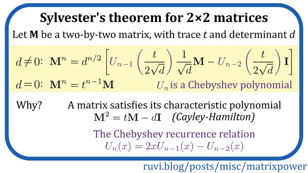
Cayley-Hamilton theorem #
The Cayley-Hamilton theorem states that every matrix satisfies its own characteristic equation. This is a powerful result with many applications, and we will see that it imposes strong constraints on the form of . I will just state the theorem, as there are many proofs avaiable online.
The characteristic equation of a matrix is the polynomial that determines its eigenvalues. A matrix has eigenvalue if
We define the characteristic equation to be the function
For two-by-two matrices this is
The Cayley-Hamilton theorem says that
which gives us:
[eqCayleyHamilton]:
Note that each term has the same 'units', i.e. is proportional to the square of matrix elements. Don't let anyone tell you that physics has a monopoloy on unit checks!
There are many ways of proving this. A rough sketch of the argument I like is
- Convince yourself that [eqCayleyHamilton] is true for any diagonal matrix, and then any diagonalisable matrix.
- Diagonal matrices are dense in the set of matrices, that is to say any matrix can be approximated arbitrarily well with a diagonal matrix.
- The characteristic polynomial, being a polynomial, is continuous. Thus if are a sequence of diagonal matrices which converge to , we have
In two dimensions, Cayley-Hamilton lets us replace squares of a matrix with a sum of linear terms . In dimensions it lets us replace with a sum of terms of order .
Chebyshev polynomials #
For the general version of Sylvester's theorem, the coefficients turn out to be a type of special function called Chebyshev polynomials, which we will introduce here.
Special functions often come across as intimidating, which I think is partly because people don't quite know how to approach them. I recommend that you look at a special function the same way you look at conventional 'special functions' like sine and cosine. You probably don't know how to find the numeric value of , and I doubt you lose any sleep over it. And while sine does have a polynomial representation as an infinite sum, that's something you only pull out in emergencies. To use trigonometric functions all you need is a rough feel for how they behave, and to know simple relations like their derivatives, and formulae such as . Aim for the same sort of understanding with special functions.
Like sine and cosine, special functions often come in pairs. For Chebyshev polynomials, these are straightforwardly named Chebyshev polynomials of the first kind and Chebyshev polynomials of the second kind. We are only interested in the second kind, which are typically denoted . Here is an integer, which is there because there are an infinite family of Chebyshev polynomials. is an -th order polynomial.
The first few Chebyshev polynomials of the second kind are
but don't spend too much on the particular polynomial form. What will be useful to us is their recurrence relation
[eqChebyshevRecurrence]:
An explicit representation for Chebyshev polynomials can be given using trigonometric functions. If we write
then the Chebyshev polynomials are given by
[eqChebyshevTrigForm]:
For the numerator is , and the right-hand side is indeed a function of . This is true for all . If you peek back at [eqSylvestersTheorem], you may have a hint at where this article is going.
Armed with Chebyshev polynomials, we can now state the generalised Sylvester's theorem. I found this in [BR20], though no proof was given. Suppose is any two-by-two non-singular matrix, with determinant and trace . Then for an integer:
[eqGeneralSylvester]:
where is the th Chebyshev polynomial. We'll see later that for singular matrices there is an even simpler formula.
In the case where has unit determiant , this reduces to
You can verify yourself that if we use the explicit form [eqChebyshevTrigForm], this will reproduce [eqSylvestersTheorem].
Proving the generalised Sylvester's theorem #
Suppose is a two-by-two matrix, with trace and derivative:
Let's make our lives simpler, and get rid of the determinant by defining
assuming the determinant is nonzero. Then we will have
With this, Cayley-Hamilton becomes
We can now derive a formula for , and then work out
Zero determinant #
Before we continue, let's quickly see what happens when has zero determinant. Cayley-Hamilton gives us
from which we find
Continuing in this way we find
Thus powers of two-by-two singular matrices take a very simple form!
Unit determinant #
Let's now try and find a formula for . The first power is trivial
while Cayley-Hamilton gives us the second power.
Now let's look at the third power. We begin by substituting the equation for the second power:
Substituting again the equation for the second power gives
Now we start to get an inkling of what's going on underneath Sylvester's theorem. Continuing in this way, we can see that Cayley-Hamilton guarantees that we will always have
for as-yet undetermined coefficients .
We want a formula that gives us . As a first step, let's find how these depend on . We have
and using Cayley-Hamilton gives
At the same time we know
Equating these gives
We can substitute the second equation into the first to get rid of .
From the above we have
where satisfies the recurrence relation
To prove Sylvester's theorem, we need to solve the relation for the coefficients .
Solving recurrence relations is as broad a topic as solving differential equations. I'm not very familiar with this subject, if someone knows any nice solutions methods please let me know. One way is to see if the recurrence relation matches a well-known form. Let's compare with [eqChebyshevRecurrence], which we can write as
This is very close, apart from the factor of two. We want , which can be solved by taking . Thus the recurrence relation is solved by
where is any integer. To find the value of , we have to use initial conditions. We know
which gives
This is satisfied by taking .
This is our solution! You can verify that this re-produces [eqGeneralSylvester]
Alternatively we could use a computational package. Mathematica's RSolve[] is able to find the solution
This is in fact another explicit representation of the Chebyshev polynomials.
For an alternate proof by induction in the case, see Jean Marie's Stackexchange answer.
Discussion #
We've found simple formulae for the powers of two-by-two matrices. Let and . If we have
where is a generalised Chebyshev polynomial of the second kind. If the determinant of is zero then the formula is even easier:
This seems incredible to me! Since the matrix elements can be complex, a two-by-two matrix has eight degrees of freedom. You would think that very little could be said about the powers of a matrix in general, without knowing more about the elements. However, we have these simple formulae that is always a linear combination of and , with the coefficients depending only on the trace and determinant. Fundamentally this follows from the Cayley-Hamilton theorem, which places strong restrictions on how complicated powers of matrices can be.
I mentioned that there are many proofs of Cayley-Hamilton, from both algebraic and analytic viewpoints. I recommend you pick your favourite proof, find the 'essential idea' of it, and then try and intuitively see how that idea constrains powers of matrices. This sort of thing can help you appreciate the amazing connections that lie between the many different areas of mathematics.
I think this gives a neat way to analytically solve recurrence relations, by comparing them with the recurrence relations of special functions. Hopefully this will come in useful in the future.
Here are some miscellaneous things I'm curious about, if you know anything about them please let me know:
- It would be interesting to look at generalisations beyond two-dimensions, and to non-integer powers.
- Can we better understand why Chebyshev polynomials, and not some other function, show up in this problem? The direct reason is the recurrence relation. But can we get a more intuitive picture?
If you have any comments or questions feel free to drop me a line at me@ruvi.blog, and you can follow me @ruvi_l.
Also, the correct pronunciation is apparently "Chebyshov".
References #
[S10] Svelto, Orazio (2010) Principles of lasers (5th edition) Springer.
[BR20] Brandi, P., & Ricci, P. E. (2020) Composition identities of Chebyshev polynomials, via 2× 2 matrix powers Symmetry, 12(5), 746.