This is a guest post by Andrew Jamieson, based on a problem we solved together.
Introduction #
Suppose you are racing in on dimension, trying to get from 0 to 1 as quickly as possible. You start with a speed of 1. However at any time you choose, you may press a button that will instantly teleport you back to the origin, and multiply your speed by , where is the location at which you pressed the button.
If you can press this button as many times as you like, how fast can you finish the race, and when are the optimal times to press this? And how do things change if the multiplier is instead ?
This question came up while thinking about traditional idle video games in which you can spend resources and purchase upgrades to increase your resource gathering rate, however these can generally only be activated by pressing restart and sacrificing all your resources.
Exploration #
To solve this problem, it pays to do a bit of exploratory analysis.
To Press or Not to Press? #
The first question that needs answering is whether it is worth pressing the button at all? To work this out, we can consider a simplified model where we plan to press the button exactly once at point r. In this case the total time taken to complete the race is
- The time taken to travel a distance while travelling at a speed of :
- The time taken to travel from the origin to while travelling at :
Adding these together gives the total time:
[eqTimeOnePress]:
We can find the optimal by solving for when the derivative is zero:
This happens when
which has solution given by the quadratic formula:
One of these solutions is negative, so not relevant to our problem. The positive solution is
Substituting this into [eqTimeOnePress] then gives a time of
This is less than 1, so it clearly does pay to press the button at least once. Now the question gets more complicated. How many times should we press the button, and when should we do so?
Multiple presses #
Now let's consider multiple presses. For reasons that will make sense later, I'm going to number the presses counter intuitively. The location of the last press will be denoted , the one immediately before that will be , and so on and so forth. The total time taken when using presses will be denoted by .
To start with, we'll assume two presses while we build some intuition for the problem. The total time to complete the race becomes:
- The time to travel until the first press at with speed :
- The time taken to travel until the second press at with speed :
- The time taken to travel from to with speed :
Adding these together gives the total time for two presses:
[eqTimeTwoPresses]:
Now optimising this using derivatives is a multivariate calculus problem that would be a pain to do by hand. But you can fire up Python or Mathematica to get a numerical solution (see the appendix for code):
The last press, , is at the same place as when we were only using one press! This is quite surprising. Let's try again with three presses and see if the pattern continues. In this case the total time is
[eqTimeThreePresses]:
and the optimal times are
Clearly this pattern is continuing. Why? Surely it would make sense that optimising across multiple presses would require adjusting all of them, not just the newest one.
Well let's take a look at equations for the times . In the case of a single press, what would happen if we started at a different speed, say ? Well then [eqTimeOnePress] becomes:
This however is only a scaling factor. Scaling factors don't change the location of the optimal point, meaning the location of the press does not depend on the incoming speed.
Now let's re-examine [eqTimeTwoPresses] by cleverly factorising it:
Remember that is the first press, and the second. Due to the scaling argument we made above, the optimal location for the second press is completely independent of the first press . However from this formula, is determined by due to the in the equation above.
Similarly for [eqTimeTwoPresses]:
This confirms the observations that seemed strange before. It turns out that the optimal press value can be calculated purely based on the optimal press values that come after it, and not those before it. Hopefully now you can see why we chose that indexing system.
Optimal solution #
Sequential formula #
Generalising the analysis in the previous section, we have the result:
[eqGeneralisedSequence]:
Solving for the optimal point when the derivative is zero, and once-again exluding a non-physical solution, gives
[eqGeneralisedRestarts]:
[eqGeneralisedSequence] and [eqGeneralisedRestarts] together can be used to generate the infinite set of every restart. Here are the first ten:
General solution and time #
At this point, it's reasonable to investigate how the speed multiplier affects the results, rather than just looking at . For this we can use the generalised form of [eqGeneralisedSequence]: :
Once again solving for optimal point at zero derivative gives:
Combining these gives us
which simplifies to
[eqGeneralisedCombined]:
In the figure below we plot for values of ranging from to (including decimals). See the appendix for Python and Mathematica code to generate this.
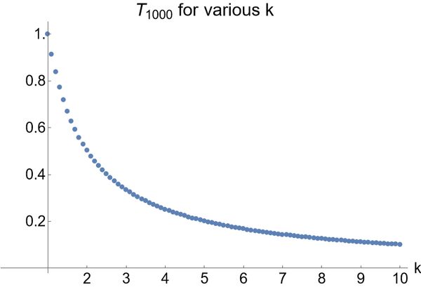
This seems very well-behaved! Motivated by this if we investigate a bit closer, when looking at the actual values, a suspicious looking pattern of the total optimal time required to complete the race is revealed:
To see whether this pattern is real, we just need to solve for the total time taken when using infinitely many presses, which can be done by taking the limit of both sides of [eqGeneralisedCombined].
Let's solve this for :
This has solution:
Conclusion #
The answer to the problem is that you should press the button, and the more times you press it the faster you can complete the race. For greater than , the formula below can be used to find the time taken, and optimal places to stop:
However, as the number of presses increases, there are diminishing returns. In the limit of infinite presses, the total time taken to complete the race will approach .
It is worth thinking about how we found the solution. To get an initial feel for the problem we did some numerical searches. These revealed a pattern in the solution, that the stopping locations for stops were the same as the times for stops (with one more added). This made the problem much easier to solve analytically, since we only had to worry about one stopping location at a time. It's always nice to see numerics inform analytics, and vice versa.
A formula like above, expressing in terms of , is called a recurrence relation. A natural question to ask is if we can solve this, and obtain a formula for in terms of just alone. Unfortunately this recurrence relation is nonlinear due to the square root term . Much like nonlinear differential equations, nonlinear recurrence relations are exteremely difficult to solve, and we usually have to resort to numerics. It is unlikely that an explicit formula exists, though please let us know if you find one or have any ideas!
Appendix #
Here you'll find Mathematica and Python code you can use to reproduce results from this article.
Finding the stopping times #
These codes compute the stopping times for a fixed number of stops.
Python #
import math

import matplotlib.pyplot as plt
import numpy as np
import scipy

def total_time_with_restarts(r, k):
    """Calculates the total time taken to complete the race given
    the location of restarts and the multiplication parameter k.

    Variables:
    r: iterable of numbers representing the location of the restart
    k: multiplication parameter"""
    sum_list = []
    for i in range(len(r)):
        divisor = []
        for j in range(i):
            divisor.append(1+k*r[j])
        sum_list.append(r[i] / math.prod(divisor))
    sum_list.append(1/math.prod((1+k*r[j] for j in range(len(r)))))
    return sum(sum_list)

k=2
for number_of_restarts in range(1, 11):
    opt = scipy.optimize.minimize(total_time_with_restarts,
      0.2 * np.ones(number_of_restarts), args=(k,),
      bounds=[(0,1) for _ in range(number_of_restarts)])
    #Prints the total optimal time along with the location
    # of the restarts in press order.
    print(number_of_restarts, total_time_with_restarts(opt.x,k), opt.x)
Mathematica #
(* Formula for the time given nR stops *)
time[nR_] :=
  Sum[If[j > 0, r[j], 1]/
   Product[1 + 2 r[nR - i + 1], {i, 1, nR - j}], {j, nR, 0, -1}];

(* Bounds on the numerical optimisation *)
bounds[nR_] := Table[0 <= r[j] <= 1, {j, 1, nR}];

(* Numerically minimise time[nR] *)
min[nR_] :=
  FindMinimum[Reverse@Append[bounds[nR], time[nR]],
   Table[r[j], {j, 1, nR}]];

(* First ten stopping times *)
Last /@ Last@min[10]
Computing T1000 #
Here is code you can use to compute and plot the for various .
Python #
import math

import matplotlib.pyplot as plt
import numpy as np
import scipy

def optimal_time(k, presses):
    """Returns the optimal race completion time given the
    multiplication factor and numer of button presses used.

    Variables:
    k: multiplication parameter
    presses: number of button presses."""
    if k == 0:
        return 1
    time=1
    for _ in range(10000):
        r = (math.sqrt(k)*math.sqrt(time) - 1)/k
        r = r if r>0 else 0
        time = r + time/(1+k*r)
    return time

presses = 1000
inputvec = [n/100 for n in range(0, 1000)]
plt.plot(inputvec, [optimal_time(k, presses) for k in inputvec])
plt.xlabel("k")
plt.ylabel("Total Time")
Mathematica #
(* Find T_(n+1) given T_n and k. *)
(* You want a . after 2 so it evaluates numerically,
   which is much faster than exact evaluation *)
Tnp1[Tn_, k_] := (-1 + 2. Sqrt[k Tn])/k;

(* Compute T_1000 by Nesting T_(n+1) 1000 times *)
(* Use a Table to do this for all k *)
T1000Data = Table[{k, Nest[Tnp1[#, k] &, 1, 1000]}, {k, 1, 10, 0.1}];

(* Plot the T_1000 *)
ListPlot[T1000Data, AxesLabel -> {"k", None},
 PlotLabel -> "T1000 for various k",
 LabelStyle -> Directive[FontSize -> 20, FontColor -> Black],
 ImageSize -> Large, Ticks -> {Range[10], Range[0.2, 1, 0.2]},
 AxesOrigin -> {1, 0}]